The Exponentially Weighted Moving Average Method
- The successful use of value at risk models is critically dependent
upon estimates of the volatility of underlying prices. The principal difficulty
is that the volatility is not constant over time - if it were, it could
be estimated with very high accuracy by using a sufficiently long sample
of data. Thus models of time varying volatility become very important.
Practitioners have often dealt with time varying parameters by confining
attention to the recent past and ignoring observations from the distant
past. Econometricians have on the other hand developed sophisticated models
of time varying volatility like the GARCH (Generalised Auto-Regressive
Conditional Heteroscedasticity) model.
Straddling the two are the exponentially weighted moving average (EWMA) methods popularised by J. P. Morgans RiskMetricsÒ system. EWMA methods can be regarded as a variant of the practitioners idea of using only the recent past because the practitioners idea is essentially that of a simple moving average where the recent past gets a weight of one and data before that gets a weight of zero. The variation in EWMA is that the observations are given different weights with the most recent data getting the highest weight and the weights declining rapidly as one goes back. Effectively, therefore, EWMA is also based on the recent past, in fact, it is even more responsive than the simple moving average to sudden changes in volatility. EWMA can also be regarded as a special case of GARCH in which the "persistence parameter" is set to unity. This means that unlike GARCH, EWMA does not have a notion of long run volatility at all and is therefore more robust under regime shifts
EWMA is computationally very simple to implement (even simpler than
a simple moving average). The volatility at the end of day t, st
is estimated using the previous volatility estimate st-1
(as at the end of day t-1),and the return rt observed in the
index during day t:
(st)2 = l
(st-1)2 + (1 - l
) (rt)2
where l is a parameter which determines how
rapidly volatility estimates change.
Whatever intuitive or theoretical merits a value at risk model may have, the ultimate test of its usability is how well it holds up against actual data. For example, tentative results indicate that foreign exchange markets in India are best modelled by processes that allow jumps and that EWMA methods do not perform well in that market at all. Empirical tests of the EWMA model in the Indian stock market are therefore of great importance. The EWMA model was therefore tested using historical data on the Indian stock market indices - the NSE-50 Index (Nifty) and the BSE-30 Index (Sensex).
Sample Period
- The data period used is from July 1, 1990 to June 30, 1998. The long
sample period reflects the view that risk management studies must attempt
(wherever possible) to cover at least two full business cycles (which would
typically cover more than two interest rate cycles and two stock market
cycles). It has been strongly argued on the other hand that studies must
exclude the securities scam of 1992 and must preferably confine itself
to the period after the introduction of screen based trading (post 1995).
- The usual definition of return as the percentage change in price has
a very serious problem in that it is not symmetric. For example, if the
index rises from 1000 to 2000, the percentage return would be 100%, but
if it falls back from 2000 to 1000, the percentage return is not -100%
but only -50%. As a result, the percentage return on the negative side
cannot be below -100%, while on the positive side, there is no limit on
the return. The statistical implication of this is that returns are skewed
in the positive direction and the use of the normal distribution becomes
inappropriate.
- The EWMA method requires the specification of the value of l
. One can estimate l itself statistically by
the method of maximum likelihood. This process yielded an estimate for
l
of 0.923 for the Nifty and 0.929 for the Sensex. These values are not statistically
significantly different from the value of 0.94 for l
used in J. P. Morgans RiskMetricsÒ system
for daily horizons. (The likelihood ratio test gives chi-squares with 1
df of 1.89 for the Sensex and 4.46 for the Nifty which are not significant
at the 1% level even though we have a sample size of over 1750). The analysis
was therefore carried out using a l of 0.94
to permit easier comparability and facilitate further extensions to the
model.
- It is well known that stock market returns are not normally distributed
even if one uses logarithmic returns to induce symmetry. However, the time
varying volatility itself is one major cause for non-normality. It is to
be expected therefore that the "conditional distribution" of the return
given the volatility estimate is approximately normal. In other words,
the return on each day divided by the estimated standard deviation for
that day should be roughly normally distributed. The results do indicate
significant reduction in non normality. The unconditional distribution
has an excess kurtosis of 5.42 for Nifty and 4.77 for Sensex while the
"conditional distribution" has an excess kurtosis of only 1.75 for Nifty
and 1.13 for Sensex. Thus over two-thirds of the excess kurtosis is eliminated
by the time varying volatility estimation process.
- Since the volatility estimates are for the logarithmic return, the
±
3 s limits for a 99% VAR would specify the maximum/minimum
limits on the logarithmic returns not the percentage returns. To convert
these into percentage margins, the logarithmic returns would have to be
converted into percentage price changes by reversing the logarithmic transformation.
Therefore the percentage margin on short positions would be equal to 100(exp(3st)-1)
and the percentage margin on long positions would be equal to 100(1-exp(-3st)).
This implies slightly larger margins on short positions than on long positions,
but the difference is not significant except during periods of high volatility
where the difference merely reflects the fact that the downside is limited
(prices can at most fall to zero) while the upside is unlimited.
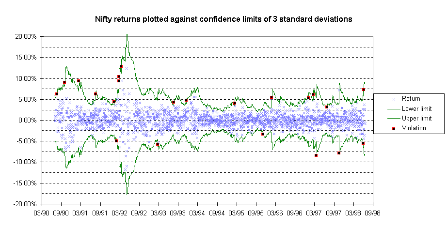
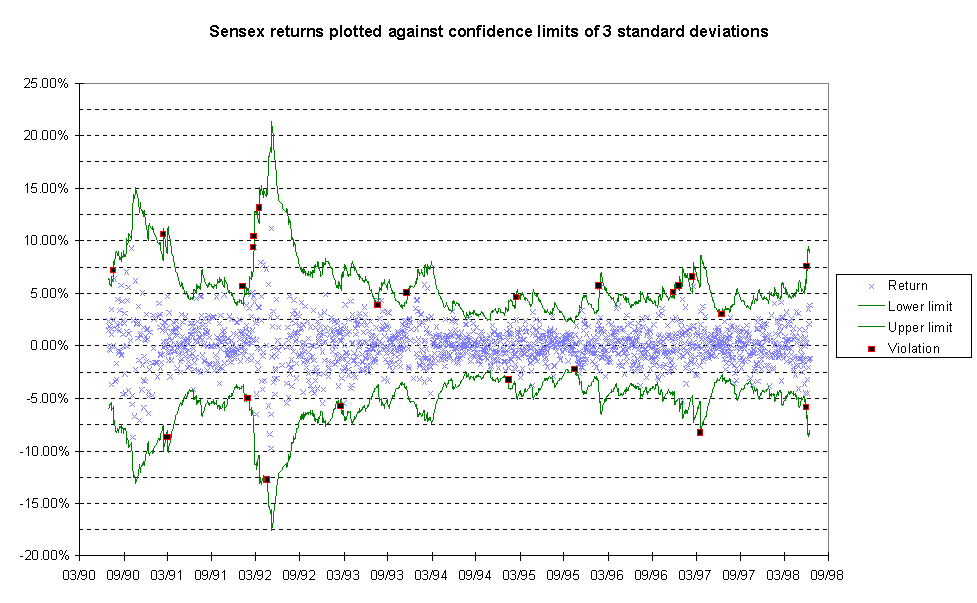
- Backtesting this model for the period over a 8 year period showed that
the 1% VAR limit was crossed 22 times in the case of Nifty and 23 times
in the case of Sensex as against the expected number of 18 violations.
The hypothesis that the true probability of a violation is 1% cannot be
rejected at even the 5% level of statistical significance though we have
a sample size of over 1750. The actual number of violations is therefore
well within the allowable limits of sampling error. In the terminology
of the Bank for International Settlements ("Supervisory framework for the
use of backtesting in conjunction with the internal models approach to
marker risk capital requirements", Basle Committee on Banking Supervision,
January 1996), these numbers are well within the "Green Zone" where the
"test results are consistent with an accurate model, and the probability
of accepting an inaccurate model is low".
The market movements, margins and margin shortfalls are shown graphically in Figures 1 and 2. The summary statistics about the actual margins on the sell side are tabulated below while year by year details of the sell side and buy side margins are given in Tables 1 and 2.
| Sell Side Margins | Nifty | Sensex |
| Average | 5.49% | 5.74% |
| Maximum | 21.73% | 21.31% |
| Minimum | 2.04% | 2.21% |
| Frequency Distribution | ||
| Below 5% | 52.51% | 50.45% |
| 5 to 10% | 41.75% | 41.99% |
| 10 to 15% | 4.17% | 6.08% |
| 15 to 20% | 1.35% | 1.31% |
| Above 20% | 0.23% | 0.17% |
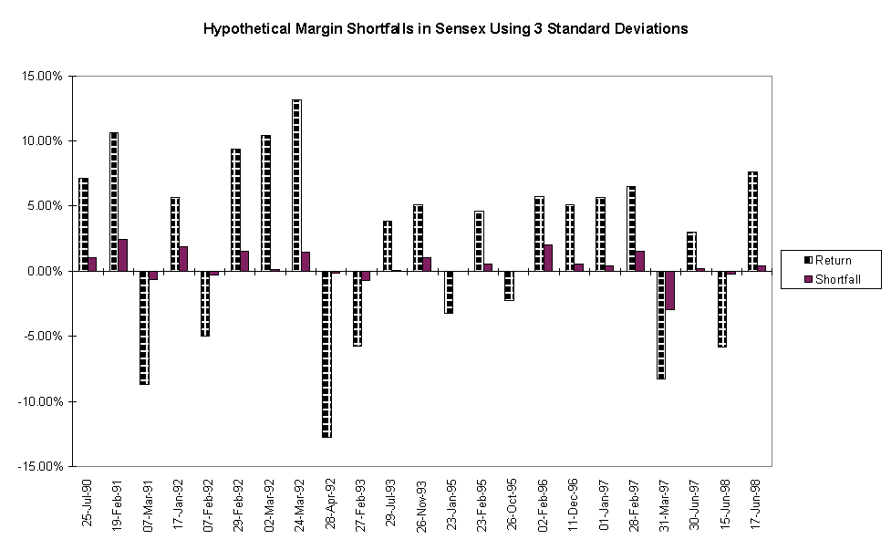
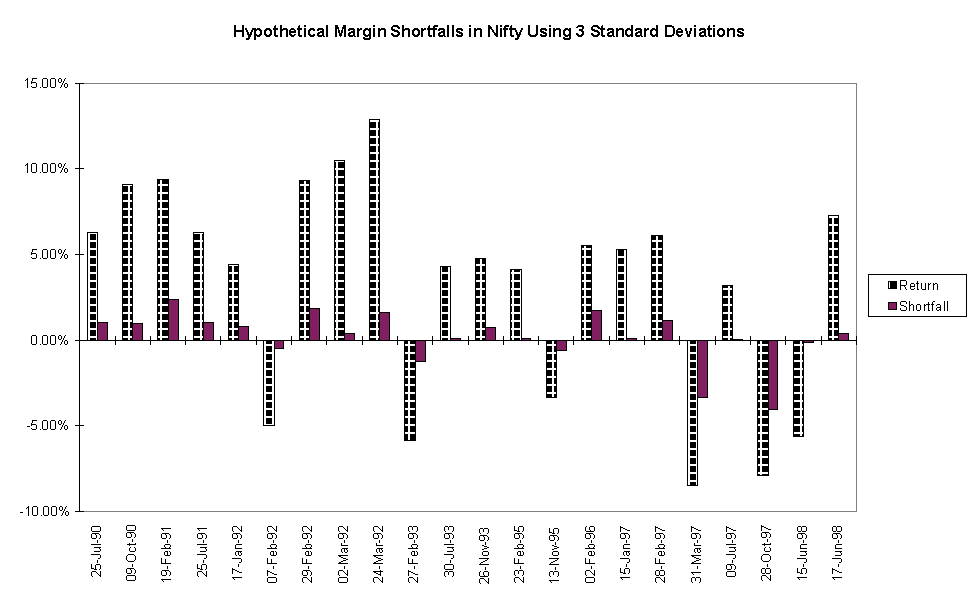
- Taking a closer look at the actual violations (See Figures 3 and 4),
it is seen that most of the violations take place when the market move
is large and the violation is typically a small fraction of the market
move. This implies that in most cases, the model is able to correctly forecast
that the markets are in a volatile period and step up the margins accordingly
to protect market integrity.
There are only two exceptions to this pattern. The first exception is March 31, 1997 when the sudden withdrawal of support to the then government by the major supporting party led to a sharp fall in the market. This is the kind of event risk which a statistical model cannot predict and against which the only protection can be a second line of defence (broker net worth). The second exception is October 28, 1997 when the global equity meltdown triggered by sharp falls in the Asian markets and in the US market drove the Indian market also down.
It is conceivable, though by no means certain, that more sophisticated
statistical models which can estimate volatility contagion across several
financial markets could have provided better protection against the market
drop of October 28, 1997. The development of multivariate models of volatility
estimation that can account for such contagion is a topic for further research.
Practical utility of such a model would however be contingent on the ability
of the derivatives exchange / clearing corporation to make a margin call
shortly before the market opens in Mumbai based on the market movement
in New York (previous day close), Tokyo (same day close) and Hong Kong
(same day morning session).
| Table 1: Summary Statistics of Margins on Nifty | ||||||||||
|
|
|
|
|
|
|
|
|
|
|
|
|
|
||||||||||
| Average |
|
|
|
|
|
|
|
|
|
|
| Maximum |
|
|
|
|
|
|
|
|
|
|
| Minimum |
|
|
|
|
|
|
|
|
|
|
| Frequency Distribution | ||||||||||
| Below 5% |
|
|
|
|
|
|
|
|
|
|
| 5 to 10% |
|
|
|
|
|
|
|
|
|
|
| 10 to 15% |
|
|
|
|
|
|
|
|
|
|
| 15 to 20% |
|
|
|
|
|
|
|
|
|
|
| Above 20% |
|
|
|
|
|
|
|
|
|
|
|
|
||||||||||
| Average |
|
|
|
|
|
|
|
|
|
|
| Maximum |
|
|
|
|
|
|
|
|
|
|
| Minimum |
|
|
|
|
|
|
|
|
|
|
| Frequency Distribution | ||||||||||
| Below 5% |
|
|
|
|
|
|
|
|
|
|
| 5 to 10% |
|
|
|
|
|
|
|
|
|
|
| 10 to 15% |
|
|
|
|
|
|
|
|
|
|
| 15 to 20% |
|
|
|
|
|
|
|
|
|
|
| Above 20% |
|
|
|
|
|
|
|
|
|
|
| Table 2: Summary Statistics of Margins on Sensex | ||||||||||
|
|
|
|
|
|
|
|
|
|
|
|
|
|
||||||||||
| Average |
|
|
|
|
|
|
|
|
|
|
| Maximum |
|
|
|
|
|
|
|
|
|
|
| Minimum |
|
|
|
|
|
|
|
|
|
|
| Frequency Distribution | ||||||||||
| Below 5% |
|
|
|
|
|
|
|
|
|
|
| 5 to 10% |
|
|
|
|
|
|
|
|
|
|
| 10 to 15% |
|
|
|
|
|
|
|
|
|
|
| 15 to 20% |
|
|
|
|
|
|
|
|
|
|
| Above 20% |
|
|
|
|
|
|
|
|
|
|
|
|
||||||||||
| Average |
|
|
|
|
|
|
|
|
|
|
| Maximum |
|
|
|
|
|
|
|
|
|
|
| Minimum |
|
|
|
|
|
|
|
|
|
|
| Frequency Distribution | ||||||||||
| Below 5% |
|
|
|
|
|
|
|
|
|
|
| 5 to 10% |
|
|
|
|
|
|
|
|
|
|
| 10 to 15% |
|
|
|
|
|
|
|
|
|
|
| 15 to 20% |
|
|
|
|
|
|
|
|
|
|
| Above 20% |
|
|
|
|
|
|
|
|
|
|

Figure 1

Figure 2

Figure 3
